'youve probably heard this quote ,'dont judge a book by its cover' .
and how does it relate to the topic ,
well , this is a matlab script from a video i found on youtube on convolutional neural network with MATLAB but for the newbies what is convolutional neural network , well in layman/simpler terms it just means training a computer to identify patterns and things , esentially giving the computer a human brain.
In even simpler terms,getting a computer to 'judge a book by its cover'.
this is the result,


now this code trains the computer to recognize a set of dataset called the mnist dataset,this is a data set consisting of handwritten numbers .
Softmax
function
Function
y= Softmax(x)
%UNTITLED6
Summary of this function goes here
% Detailed explanation goes here
Ex =
exp(x);
Y
=ex/sum(ex);
End
Explanation
This is a
function that takes an input vector `x` and applies the Softmax function to it.
The Softmax function is commonly used in the output layer of a neural network
for multi-class classification problems. It converts the input vector into a
probability distribution over the classes.
1.
`function y= Softmax(x)` This line defines
the function signature, specifying that it takes one input argument `x` and
returns one output argument `y`.
2.
`ex = exp(x);` This line calculates the
element-wise exponential of the input vector `x` and stores the result in a new
variable called `ex`.
3.
`y =ex/sum(ex);` This line calculates the
element-wise division of `ex` by the sum of its elements, and stores the result
in the output variable `y`.
4.
`end` This line marks the end of the
function definition.
Relu
Function y
= ReLU(x)
%UNTITLED5
Summary of this function goes here
% Detailed explanation goes here
Y =
max(0,x);
End
Explanation
This is a
function that takes an input `x` and applies the Rectified Linear Unit (ReLU)
function to it. The ReLU function is a commonly used activation function in
neural networks, defined as `f(x) = max(0, x)`.
1.
`function y = ReLU(x)` This line defines
the function signature, specifying that it takes one input argument `x` and
returns one output argument `y`.
2.
`y = max(0,x);` This line calculates the
element-wise maximum of 0 and the input `x`, and stores the result in the
output variable `y`.
3.
`end` This line marks the end of the
function definition.
Pool.m
Function y
= Pool( x )
%UNTITLED8
Summary of this function goes here
% Detailed explanation goes here
[xrow,xcol,numFilters]
= size(x);
Y =
zeros(xrow/2, xcol/2,numFilters);
For k =
1:numFilters
Filter = ones(2)/(2*2);
Image = conv2(x(:, :,k),filter,’valid’);
Y(:, :, k) = image(1:2:end,1:2:end);
End
End
Explanation
This is a
function that takes an input `x` and applies a 2x2 average pooling operation to
it. Pooling is a common operation in convolutional neural networks that reduces
the spatial dimensions of the input by taking the average or maximum value over
a small region.
1.
`function y = Pool( x )` This line defines
the function signature, specifying that it takes one input argument `x` and
returns one output argument `y`.
2.
`[xrow,xcol,numFilters] = size(x);` This
line gets the size of the input `x`, which is assumed to be a 3D array with
dimensions [height, width, numFilters], and stores the values in variables
`xrow`, `xcol`, and `numFilters`.
3.
`y = zeros(xrow/2, xcol/2,numFilters);`
This line initializes the output variable `y` as a 3D array of zeros with
dimensions [height/2, width/2, numFilters].
4.
The next block of code is a for loop that
runs for each filter:
-
`for k = 1:numFilters`
-
`filter = ones(2)/(2*2);` This line
creates a 2x2 filter of ones and divides it by 4 to get an average filter.
-
`image = conv2(x(:, :,k),filter,’valid’);`
This line applies 2D convolution between the k-th slice of the input `x` and
the filter, using the ‘valid’ option to discard border pixels.
-
`y(:, :, k) = image(1:2:end,1:2:end);`
This line downsamples the resulting image by taking every other pixel along
both dimensions, and stores it in the k-th slice of the output variable `y`.
-
`end`
5.
`end` This line marks the end of the
function definition.
The
resulting value `y` is the result of applying 2x2 average pooling to each slice
of the input `x`.
Plot
features.m
Load(‘MnistConv.mat’)
K = 1;
X = X(:, :,k);
Y1 = Conv(x,W1);
Y2 = ReLU(y1);
Y3 = Pool(y2);
Y4 = reshape(y3,[],1);
V5 = W5*y4;
Y5 = ReLU(v5);
V = Wo *y5;
Y = Softmax(v);
Figure;
Display_network(x(J);
Title(‘input image’)
convFilters = zeros(9*9,20);
for i = 1:20
filter = W1(:,:,i);
convFilters(:,i) = filter(J;
end
figure
display_network(convFilters);
title(‘Convolution filters’)
flist = zeros(20*20,20);
for i = 1:20
feature = y1(:, :, i);
flist(:,i) = feature(J;
end
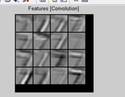
figure
display_network(flist);
title(‘Features [Convolution]’)
flist = zeros(20*20,20);
for i = 1:20
feature = y2(:, :, i);
flist(:,i) = feature(J;
end
figure
display_network(flist);
title(‘Features [Convolution+ReLU]’)
flist = zeros(20*20,20);
for i = 1:20
feature = y3(:, :, i);
flist(:,i) = feature(J;
end
figure
display_network(flist);
title(‘Features
[Convolution+ReLU+Meanpool]’)
flist = zeros(20*20,20);
for i = 1:20
feature = y3(:, :, i);
flist(:,i) = feature(J;
end
explanation
This
script loads the trained weights of a convolutional neural network from a file
called ‘MnistConv.mat’ and visualizes the input image, the convolutional
filters, and the features at different layers of the network for a single
image.
1.
`load(‘MnistConv.mat’)` This line loads
the trained weights `W1`, `W5`, and `Wo` from a file called ‘MnistConv.mat’.
2.
`k = 1;` This line sets the index of the
image to visualize to 1.
3.
The next block of code performs forward
propagation through each layer of the network for the selected image:
-
`x = X(:, :,k);`
-
`y1 = Conv(x,W1);`
-
`y2 = ReLU(y1);`
-
`y3 = Pool(y2);`
-
`y4 = reshape(y3,[],1);`
-
`v5 = W5*y4;`
-
`y5 = ReLU(v5);`
-
`v = Wo *y5;`
-
`y = Softmax(v);`
4.
The next block of code visualizes the
input image:
-
`figure;` This line creates a new figure
window.
-
`display_network(x(J);` This line
calls the function `display_network` to display the input image as a grayscale
image.
-
`title(‘input image’)` This line adds a
title to the figure.
5.
The next block of code visualizes the
convolutional filters:
-
`convFilters = zeros(9*9,20);` This line
initializes a variable called ‘convFilters’ as a 2D array of zeros with
dimensions [81, 20].
-
The next block of code is a for loop that
runs for each filter:
-
`for i = 1:20`
-
`filter = W1(:,:,i);` This line selects
the i-th filter from variable ‘W1’ and stores it in a new variable called ‘filter’.
-
`convFilters(:,i) = filter(J;` This
line reshapes the filter into a column vector and stores it in the i-th column
of variable ‘convFilters’.
-
`end`
-
`figure` This line creates a new figure window.
-
`display_network(convFilters);` This line
calls the function ‘display_network’ to display the convolutional filters as
grayscale images.
-
`title(‘Convolution filters’)` This line
adds a title to the figure.
6.
The next block of code visualizes the features
after the first convolutional layer:
-
`flist = zeros(20*20,20);` This line
initializes a variable called ‘flist’ as a 2D array of zeros with dimensions
[400, 20].
-
The next block of code is a for loop that
runs for each feature map:
-
`for i = 1:20`
-
`feature = y1(:, :, i);` This line selects
the i-th feature map from variable ‘y1’ and stores it in a new variable called ‘feature’.
-
`flist(:,i) = feature(J;` This
line reshapes the feature map into a column vector and stores it in the i-th
column of variable ‘flist’.
-
`end`
7.
The next block of code visualizes the
features after the ReLU activation function:
-
`figure` This line creates a new figure
window.
-
`display_network(flist);` This line calls
the function ‘display_network’ to display the feature maps as grayscale images.
-
`title(‘Features [Convolution+ReLU]’)`
This line adds a title to the figure.
8.
The next block of code visualizes the
features after the pooling layer:
-
`flist = zeros(20*20,20);` This line
initializes a variable called ‘flist’ as a 2D array of zeros with dimensions
[400, 20].
-
The next block of code is a for loop that
runs for each feature map:
-
`for i = 1:20`
-
`feature = y3(:, :, i);` This line selects
the i-th feature map from variable ‘y3’ and stores it in a new variable called ‘feature’.
-
`flist(:,i) = feature(J;` This
line reshapes the feature map into a column vector and stores it in the i-th
column of variable ‘flist’.
-
`end`
-
`figure` This line creates a new figure
window.
-
`display_network(flist);` This line calls
the function ‘display_network’ to display the feature maps as grayscale images.
-
`title(‘Features
[Convolution+ReLU+Meanpool]’)` This line adds a title to the figure.
MnistConv.m
Function [
W1,W5,Wo ] = MnistConv( W1,W5,Wo ,X,D )
%UNTITLED9
Summary of this function goes here
% Detailed explanation goes here
Alpha =
0.01;
Beta =
0.95;
Momentum1
= zeros(size(W1));
Momentum5
= zeros(size(W5));
Momentumo
= zeros(size(Wo));
N = length(D);
Bsize =
100;
Blist =
1:bsizeLN-bsize+1);
For batch
= 1: length(blist)
dW1 = zeros(size(W1));
dW5 = zeros(size(W5));
dWo = zeros(size(Wo));
begin = blist(batch);
for k = begin:begin+bsize-1
x = X(:, :,k);
y1 = Conv(x,W1);
y2 = ReLU(y1);
y3 = Pool(y2);
y4 = reshape(y3,[],1);
v5 = W5*y4;
y5 = ReLU(v5);
v = Wo *y5;
y = Softmax(v);
d = zeros(10,1);
d(sub2ind(size(d),D(k),1)) = 1;
e = d-y;
delta = e;
e5 = Wo’ * delta;
delta5 = (y5>0) .* e5;
e4 = W5’ * delta5;
e3 = reshape(e4,size(y3));
e2 = zeros(size(y2));
W3 = ones(size(y2)) / (2*2);
For c = 1:20
E2 (:, :, c) = kron(e3(:, :,
c),ones([2,2])).*W3(:, :,c);
End
Delta2 = (y2>0).*e2;
Delta1_x = zeros(size(W1));
For c = 1:20
Delta1_x(:, :, c) = conv2(x(:, J,rot90(delta2(:,
:, c),2),’valid’);
End
dW1 = dW1 + delta1_x;
dW5 = dW5 +delta5*y4’;
dWo = dWo +delta *y5’;
end
dW1 = dW1/bsize;
dW5 = dW5 /bsize;
dWo = dWo /bsize;
momentum1 = alpha *dW1 +beta*momentum1;
W1 = W1 + momentum1;
Momentum5 = alpha *dW5 + beta* momentum5;
W5 =
W5 +momentum5;
Momentumo = alpha *dWo +beta*momentumo;
Wo = Wo+ momentumo;
End
End
Explanation
`MnistConv.m`
is a function that performs one epoch of training on a convolutional neural
network with one convolutional layer, one fully connected layer, and an output
layer. The function takes as input the current values of the weights `W1`,
`W5`, and `Wo`, the training data `X`, and the training labels `D`. It returns
the updated values of the weights after one epoch of training.
1.
`function [ W1,W5,Wo ] = MnistConv(
W1,W5,Wo ,X,D )` This line defines the function signature, specifying that it
takes five input arguments and returns three output arguments.
2.
`alpha = 0.01;` This line sets the
learning rate to 0.01.
3.
`beta = 0.95;` This line sets the momentum
parameter to 0.95.
4.
The next three lines initialize the
momentum variables for each layer to zero:
-
`momentum1 = zeros(size(W1));`
-
`momentum5 = zeros(size(W5));`
-
`momentumo = zeros(size(Wo));`
5.
`N = length(D);` This line calculates the
number of training examples by taking the length of variable ‘D’.
6.
`bsize = 100;` This line sets the batch
size to 100.
7.
`blist = 1:bsizeLN-bsize+1);` This
line creates a list of batch start indices by taking steps of size ‘bsize’ from
1 to ‘N-bsize+1’.
8.
The next block of code is a for loop that
runs for each batch:
-
`for batch = 1: length(blist)`
-
The next three lines initialize the gradients
for each layer to zero:
-
`dW1 = zeros(size(W1));`
-
`dW5 = zeros(size(W5));`
-
`dWo = zeros(size(Wo));`
-
`begin = blist(batch);` This line gets the
start index of the current batch from variable ‘blist’.
-
The next block of code is a for loop that
runs for each example in the current batch:
-
`for k = begin:begin+bsize-1`
-
The next block of code performs forward propagation
through each layer of the network for the current example:
-
`x = X(:, :,k);`
-
`y1 = Conv(x,W1);`
-
`y2 = ReLU(y1);`
-
`y3 = Pool(y2);`
-
`y4 = reshape(y3,[],1);`
-
`v5 = W5*y4;`
-
`y5 = ReLU(v5);`
-
`v = Wo *y5;`
-
`y = Softmax(v);`
-
The next block of code computes the error
and backpropagates it through each layer of the network:
-
`d = zeros(10,1);` This line initializes a
target vector ‘d’ of zeros with length 10.
-
`d(sub2ind(size(d),D(k),1)) = 1;` This
line sets the element of ‘d’ corresponding to the true class label to 1.
-
`e = d-y;` This line computes the error
between the target vector ‘d’ and the predicted probabilities ‘y’.
-
The next block of code backpropagates the
error through each layer of the network:
-
`delta = e;` This line sets the delta for
the output layer to the error ‘e’.
9.
The next block of code computes the
average gradients for the current batch:
-
`dW1 = dW1/bsize;` This line divides the
accumulated gradient for weights `W1` by the batch size to get the average
gradient.
-
`dW5 = dW5 /bsize;` This line divides the
accumulated gradient for weights `W5` by the batch size to get the average
gradient.
-
`dWo = dWo /bsize;` This line divides the
accumulated gradient for weights `Wo` by the batch size to get the average
gradient.
10.
The next block of code updates the weights
using momentum:
-
`momentum1 = alpha *dW1 +beta*momentum1;`
This line updates the momentum variable for weights `W1` by taking a weighted
average of the current gradient and the previous momentum value.
-
`W1 = W1 + momentum1;` This line updates
weights `W1` by adding the momentum variable to it.
-
`momentum5 = alpha *dW5 + beta*
momentum5;` This line updates the momentum variable for weights `W5` by taking
a weighted average of the current gradient and the previous momentum value.
-
`W5
= W5 +momentum5;` This line updates weights `W5` by adding the momentum
variable to it.
-
`momentumo = alpha *dWo +beta*momentumo;`
This line updates the momentum variable for weights `Wo` by taking a weighted
average of the current gradient and the previous momentum value.
-
`Wo = Wo+ momentumo;` This line updates
weights `Wo` by adding the momentum variable to it.
11.
`end` This line marks the end of the batch
loop.
12.
`end` This line marks the end of the
function definition.
Mg.m
Function
mg( x)
%UNTITLED10
Summary of this function goes here
% Detailed explanation goes here
Rng(x,
‘twister’);
End
Explanation
`mg.m` is
a function that takes an input `x` and sets the seed for the random number
generator to `x`, using the ‘twister’ algorithm.
1.
`function mg( x)` This line defines the
function signature, specifying that it takes one input argument `x`.
2.
`rng(x, ‘twister’);` This line sets the
seed for the random number generator to `x`, using the ‘twister’ algorithm.
3.
`end` This line marks the end of the
function definition.
This
function can be used to set the seed for the random number generator to a
specific value, which can be useful for reproducibility.
Loadmnistimages.m
Function
images = loadmnstimages(filename )
%UNTITLED3
Summary of this function goes here
% Detailed explanation goes here
Fp =
fopen(filename,’rb’);
Assert(fp~=-1,[‘could
not open’,filename,’’]);
Magic =
fread(fp,1,’int32’,0,’ieee-be’);
Assert(magic
== 2051, [‘Bad magic number in’,filename,’’]);
numImages
= fread(fp,1,’int32’,0,’ieee-be’);
numRows =
fread(fp,1,’int32’,0,’ieee-be’);
numCols =
fread(fp,1,’int32’,0,’ieee-be’);
images = fread(fp,inf,’unsigned char=>unsigned
char’);
images =
reshape(images,numCols,numRows,numImages);
images =
permute(images,[2 1 3]);
fclose(fp);
images =
reshape(images,size(images,1)*size(images,2),size(images,3));
images =
double(images)/255;
end
explanation
`loadmnistimages.m`
is a function that takes a filename as input and loads the MNIST images from
the specified file. The function returns the images as a 2D array, where each
column represents an image.
Here’s a
line-by-line explanation of the code:
1.
`function images = loadmnstimages(filename
)` This line defines the function signature, specifying that it takes one input
argument `filename` and returns one output argument `images`.
2.
`fp = fopen(filename,’rb’);` This line
opens the specified file in binary read mode and returns a file pointer.
3.
`assert(fp~=-1,[‘could not open’,filename,’’]);`
This line checks if the file was successfully opened and throws an error if it
was not.
4.
`magic = fread(fp,1,’int32’,0,’ieee-be’);`
This line reads the magic number from the file, which is used to identify the
file format.
5.
`assert(magic == 2051, [‘Bad magic number
in’,filename,’’]);` This line checks if the magic number is correct and throws
an error if it is not.
6.
The next three lines read the number of
images, rows, and columns from the file:
-
`numImages = fread(fp,1,’int32’,0,’ieee-be’);`
-
`numRows = fread(fp,1,’int32’,0,’ieee-be’);`
-
`numCols = fread(fp,1,’int32’,0,’ieee-be’);`
7.
`images
= fread(fp,inf,’unsigned char=>unsigned char’);` This line reads the
image data from the file as unsigned characters.
8.
`images = reshape(images,numCols,numRows,numImages);`
This line reshapes the image data into a 3D array with dimensions [numCols,
numRows, numImages].
9.
`images = permute(images,[2 1 3]);` This
line permutes the dimensions of the image data to put the rows first and columns
second.
10.
`fclose(fp);` This line closes the file.
11.
The next two lines reshape the image data
into a 2D array where each column represents an image and normalize the pixel
values to be between 0 and 1:
-
`images =
reshape(images,size(images,1)*size(images,2),size(images,3));`
-
`images = double(images)/255;`
12.
`end` This line marks the end of the
function definition.
This
function can be used to load the MNIST images from a file into a 2D array for
further processing.
loadMNISTLabels.m
function
labels = loadMNISTLabels( filename )
%UNTITLED4
Summary of this function goes here
% Detailed explanation goes here
Fp =
fopen(filename,’rb’);
Assert(fp~=-1,[‘could
not open’,filename,’’]);
Magic =
fread(fp,1,’int32’,0,’ieee-be’);
Assert(magic
== 2049, [‘Bad magic number in’,filename,’’]);
numLabels
= fread(fp,1,’int32’,0,’ieee-be’);
labels = fread(fp,inf,’unsigned char’);
assert(size(labels,1)==
numLabels,’Mismatch in label count’);
fclose(fp);
end
explanation
`loadMNISTLabels.m`
is a function that takes a filename as input and loads the MNIST labels from
the specified file. The function returns the labels as a column vector.
Here’s a
line-by-line explanation of the code:
1.
`function labels = loadMNISTLabels(
filename )` This line defines the function signature, specifying that it takes
one input argument `filename` and returns one output argument `labels`.
2.
`fp = fopen(filename,’rb’);` This line
opens the specified file in binary read mode and returns a file pointer.
3.
`assert(fp~=-1,[‘could not open’,filename,’’]);`
This line checks if the file was successfully opened and throws an error if it
was not.
4.
`magic = fread(fp,1,’int32’,0,’ieee-be’);`
This line reads the magic number from the file, which is used to identify the
file format.
5.
`assert(magic == 2049, [‘Bad magic number
in’,filename,’’]);` This line checks if the magic number is correct and throws
an error if it is not.
6.
`numLabels = fread(fp,1,’int32’,0,’ieee-be’);`
This line reads the number of labels from the file.
7.
`labels
= fread(fp,inf,’unsigned char’);` This line reads the label data from
the file as unsigned characters.
8.
`assert(size(labels,1)== numLabels,’Mismatch
in label count’);` This line checks if the number of labels read from the file
matches the expected number and throws an error if it does not.
9.
`fclose(fp);` This line closes the file.
10.
`end` This line marks the end of the
function definition.
This
function can be used to load the MNIST labels from a file into a column vector
for further processing.
Display_network.m
Function [
h,array ] = display_network(A,opt_normalize,opt_graycolor,cols,opt_colmajor)
%UNTITLED12
Summary of this function goes here
% Detailed explanation goes here
Warning
off all
If
~exist(‘opt_normalize’,’var’)|| isempty(opt_normalize)
Opt_normalize = true;
End
If
~exist(‘opt_graycolor’,’var’)|| isempty(opt_graycolor)
Opt_graycolor = true;
End
If
~exist(‘opt_colmajor’,’var’)|| isempty(opt_colmajor)
Opt_colmajor = false;
End
A = A –
mean(A(J);
If
opt_graycolor,colormap(gray);end
[L M] =
size(A);
Sz =
sqrt(L);
Buf = 1;
If
~exist(‘cols’,’var’)
If floor(sqrt(M)^2) ~= M
N = cell(sqrt(M));
While mod(M,
n)~=0&&n<1.2*sqrt(M),n = n+1;end
M = ceil(M/n);
Else
N =sqrt(M);
M = n;
End
Else
N = cols;
M = ceil(M/n);
End
Array =
-ones(buf+m*(sz+buf),(buf+n*(sz+buf)));
If
~opt_graycolor
Array = 0.1.*array;
End
If
~opt_colmajor
K=1;
For i = 1:m
For j = 1:n
If k>M,
Continue;
End
Clim = max(abs(A(:,k)));
If ~opt_normalize
Array(buf
+(i-1)*(sz+buf)+(1:sz),buf+(j-1)*(sz+buf)+(1:sz))=reshape(A(:,k),sz,sz)/clim;
Else
Array(buf
+(i-1)*(sz+buf)+(1:sz),buf+(j-1)*(sz+buf)+(1:sz))=reshape(A(:,k),sz,sz)/max(abs(A(J));
End
K = k+1;
End
End
Else
K = 1;
For i = 1:n
For j = 1:m
If k>M,
Continue;
End
Clim = max(abs(A(:,k)));
If opt_normalize
Array(buf
+(i-1)*(sz+buf)+(1:sz),buf+(j-1)*(sz+buf)+(1:sz))=reshape(A(:,k),sz,sz)/clim;
Else
Array(buf
+(i-1)*(sz+buf)+(1:sz),buf+(j-1)*(sz+buf)+(1:sz))=reshape(A(:,k),sz,sz)/max(abs(A(J));
End
K = k+q;
End
End
End
If
opt_graycolor
H = imagesc(array,’EraseMode’,’none’,[-1
1]);
Else
H = imagesc(array,’Erasemode’,’none’,[-1
1]);
End
Axis image
off
Drawnow;
Warning on
all
Explanation
`display_network.m`
is a function that takes a 2D array `A` as input, where each column represents
an image or filter, and displays the images or filters as a grid of subplots.
The function has several optional arguments that control the normalization,
color, layout, and ordering of the images or filters.
Here’s a
line-by-line explanation of the code:
1.
`function [ h,array ] =
display_network(A,opt_normalize,opt_graycolor,cols,opt_colmajor)` This line
defines the function signature, specifying that it takes five input arguments
and returns two output arguments.
2.
`warning off all` This line turns off all
warning messages.
3.
The next block of code sets default values
for the optional arguments if they are not provided:
-
`if ~exist(‘opt_normalize’,’var’)||
isempty(opt_normalize)`
-
`opt_normalize = true;`
-
`end`
-
`if ~exist(‘opt_graycolor’,’var’)||
isempty(opt_graycolor)`
-
`opt_graycolor = true;`
-
`end`
-
`if ~exist(‘opt_colmajor’,’var’)||
isempty(opt_colmajor)`
-
`opt_colmajor = false;`
-
`end`
4.
`A = A – mean(A(J);` This line
subtracts the mean of all elements in `A` from each element in `A`.
5.
`if opt_graycolor,colormap(gray);end` This
line sets the colormap to grayscale if the ‘opt_graycolor’ argument is true.
6.
`[L M] = size(A);` This line gets the size
of the input array `A`, where `L` is the number of rows and `M` is the number
of columns.
7.
`sz = sqrt(L);` This line calculates the
square root of the number of rows in `A`, which is assumed to be the height and
width of each image or filter.
8.
`buf = 1;` This line sets the buffer size
between images or filters to 1 pixel.
9.
The next block of code calculates the number
of rows and columns in the grid of subplots:
-
`if ~exist(‘cols’,’var’)`
-
The next block of code calculates the
number of rows and columns if the ‘cols’ argument is not provided:
-
`if floor(sqrt(M)^2) ~= M`
-
`n = cell(sqrt(M));`
-
The next block of code finds the smallest
integer ‘n’ that divides ‘M’:
-
`while mod(M,
n)~=0&&n<1.2*sqrt(M),n = n+1;end`
-
`m = ceil(M/n);` This line calculates the
number of rows ‘m’ by dividing ‘M’ by ‘n’.
-
`else`
-
The next block of code sets ‘n’ and ‘m’ to
be equal to the square root of ‘M’ if ‘M’ is a perfect square:
-
`n =sqrt(M);`
-
`m = n;`
-
`end`
-
The next block of code sets ‘n’ to be
equal to the value of the ‘cols’ argument if it is provided:
-
`else`
-
`n = cols;`
-
`m = ceil(M/n);` This line calculates the
number of rows ‘m’ by dividing ‘M’ by ‘n’.
-
`end`
10.
The next block of code initializes a 2D
array called ‘array’ with dimensions [buf+m*(sz+buf), buf+n*(sz+buf)] and fills
it with values of -1:
-11. `array =
-ones(buf+m*(sz+buf),(buf+n*(sz+buf)));` This line initializes a 2D array
called ‘array’ with dimensions [buf+m*(sz+buf), buf+n*(sz+buf)] and fills it
with values of -1.
11.
`if ~opt_graycolor` This line checks if
the ‘opt_graycolor’ argument is false.
12.
`array = 0.1.*array;` If the ‘opt_graycolor’
argument is false, this line scales the values in ‘array’ by a factor of 0.1.
13.
The next block of code fills the ‘array’
with the images or filters from ‘A’:
-
`if ~opt_colmajor`
-
`k=1;` This line initializes a counter
variable ‘k’ to 1.
-
The next block of code is a nested for
loop that runs for each row and column in the grid of subplots:
-
`for i = 1:m`
-
`for j = 1:n`
-
The next block of code checks if all
images or filters have been displayed:
-
`if k>M,`
-
`continue;`
-
`end`
-
The next block of code normalizes the
current image or filter and copies it into the ‘array’:
-
`clim
= max(abs(A(:,k)));` This line calculates the maximum absolute value of
the current image or filter.
-
The next block of code checks if
normalization is enabled:
-
`if ~opt_normalize`
-
`array(buf
+(i-1)*(sz+buf)+(1:sz),buf+(j-1)*(sz+buf)+(1:sz))=reshape(A(:,k),sz,sz)/clim;`
If normalization is disabled, this line normalizes the current image or filter
by dividing it by its maximum absolute value and copies it into the ‘array’.
-
`else`
-
`array(buf
+(i-1)*(sz+buf)+(1:sz),buf+(j-1)*(sz+buf)+(1:sz))=reshape(A(:,k),sz,sz)/max(abs(A(J));` If
normalization is enabled, this line normalizes the current image or filter by
dividing it by the maximum absolute value of all elements in ‘A’ and copies it
into the ‘array’.
-
`end`
-
`k = k+1;` This line increments the
counter variable ‘k’.
-
`end`
-
The next block of code fills the ‘array’
with the images or filters from ‘A’ in column-major order:
-
`else`
-
`k = 1;` This line initializes a counter
variable ‘k’ to 1.
-
The next block of code is a nested for
loop that runs for each column and row in the grid of subplots:
-
`for i = 1:n`
-
`for j = 1:m`
-
The next block of code checks if all
images or filters have been displayed:
-
`if k>M,`
-
`continue;`
-
`end`
-
The next block of code normalizes the
current image or filter and copies it into the ‘array’:
-
`clim = max(abs(A(:,k)));` This line
calculates the maximum absolute value of the current image or filter.
-
The next block of code checks if
normalization is enabled:
-
`if opt_normalize`
-
`array(buf
+(i-1)*(sz+buf)+(1:sz),buf+(j-1)*(sz+buf)+(1:sz))=reshape(A(:,k),sz,sz)/clim;`
If normalization is enabled, this line normalizes the current image or filter
by dividing it by its maximum absolute value and copies it into the ‘array’.
-
`else`
-
`array(buf
+(i-1)*(sz+buf)+(1:sz),buf+(j-1)*(sz+buf)+(1:sz))=reshape(A(:,k),sz,sz)/max(abs(A(J));` If
normalization is disabled, this line normalizes the current image or filter by
dividing it by the maximum absolute value of all elements in ‘A’ and copies it
into the ‘array’.
-
`end`
-
`k = k+q;` This line increments the
counter variable ‘k’ by ‘q’.
-
`end`
-
`end`
2.
The next block of code displays the ‘array’
as an image:
-
`if opt_graycolor`
-
`h = imagesc(array,’EraseMode’,’none’,[-1
1]);` If the ‘opt_graycolor’ argument is true, this line displays the ‘array’
as a grayscale image with values in the range [-1, 1].
-
`else`
-
`h = imagesc(array,’Erasemode’,’none’,[-1
1]);` If the ‘opt_graycolor’ argument is false, this line displays the ‘array’
as a color image with values in the range [-1, 1].
-
`end`
3.
The next two lines set the axis properties
and update the figure:
-
`axis image off`
-
`drawnow;`
4.
`warning on all` This line turns all
warning messages back on.
Conv.m
Function y
= Conv( x,W)
%UNTITLED7
Summary of this function goes here
% Detailed explanation goes here
[wrow,wcol,numFilters]
= size(W);
[xrow,xcol,~ ] = size(x);
Yrow =
xrow – wrow +1;
Ycol =
xcol -wcol +1;
Y =
zeros(yrow,ycol,numFilters);
For k = 1:
numFilters
Filter = W(:, :, k);
Filter = rot90(squeeze(filter),2);
Y(:, :, k) = conv2(x,filter,’valid’);
End
End
Explanation
This
function takes a 2D array where each column represents an image or filter and
displays the images or filters as a grid of subplots. The optional arguments
control the normalization, color, layout, and ordering of the images or
filters.
`Conv.m`
is a function that takes an input `x` and a set of filters `W` and applies 2D
convolution between `x` and each filter in `W`. The function returns the result
of the convolution as a 3D array, where each slice along the third dimension
corresponds to the result of convolving `x` with one filter.
Here’s a
line-by-line explanation of the code:
1.
`function y = Conv( x,W)` This line
defines the function signature, specifying that it takes two input arguments
`x` and `W`, and returns one output argument `y`.
2.
`[wrow,wcol,numFilters] = size(W);` This
line gets the size of the filters `W`, which is assumed to be a 3D array with
dimensions [filter_height, filter_width, numFilters], and stores the values in
variables `wrow`, `wcol`, and `numFilters`.
3.
`[xrow,xcol,~ ] = size(x);` This line gets the size
of the input `x`, which is assumed to be a 2D array with dimensions [height,
width], and stores the values in variables `xrow` and `xcol`.
4.
`yrow = xrow – wrow +1;` This line
calculates the height of the output by subtracting the filter height from the
input height and adding 1.
5.
`ycol = xcol -wcol +1;` This line
calculates the width of the output by subtracting the filter width from the
input width and adding 1.
6.
`y = zeros(yrow,ycol,numFilters);` This
line initializes the output variable `y` as a 3D array of zeros with dimensions
[output_height, output_width, numFilters].
7.
The next block of code is a for loop that
runs for each filter:
-
`for k = 1: numFilters`
-
`filter = W(:, :, k);` This line selects
the k-th filter from variable ‘W’ and stores it in a new variable called ‘filter’.
-
`filter = rot90(squeeze(filter),2);` This
line rotates the filter by 180 degrees.
-
`y(:, :, k) = conv2(x,filter,’valid’);`
This line applies 2D convolution between the input ‘x’ and the rotated filter,
using the ‘valid’ option to discard border pixels, and stores the result in the
k-th slice of the output variable ‘y’.
-
`end`
8.
`end` This line marks the end of the
function definition.
The
resulting value `y` is a 3D array where each slice along the third dimension
corresponds to the result of convolving `x` with one filter from `W.
Comments
Post a Comment